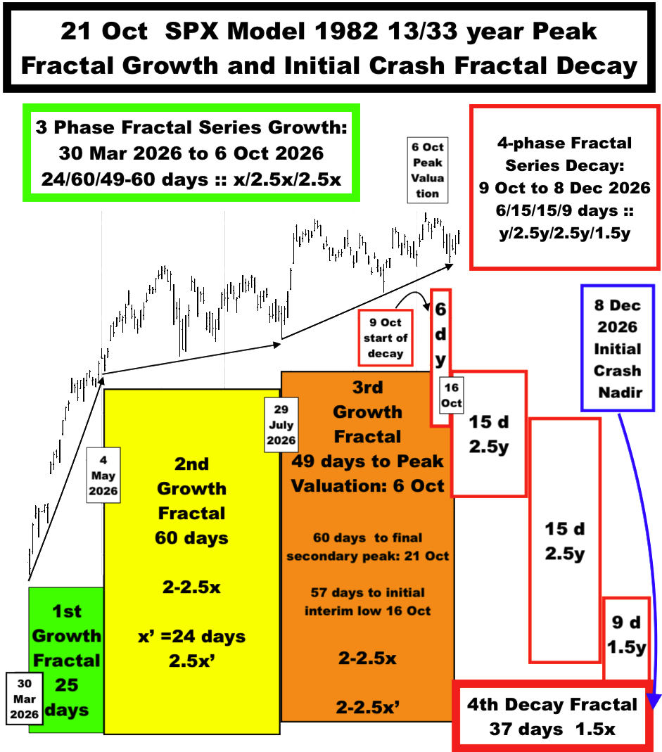
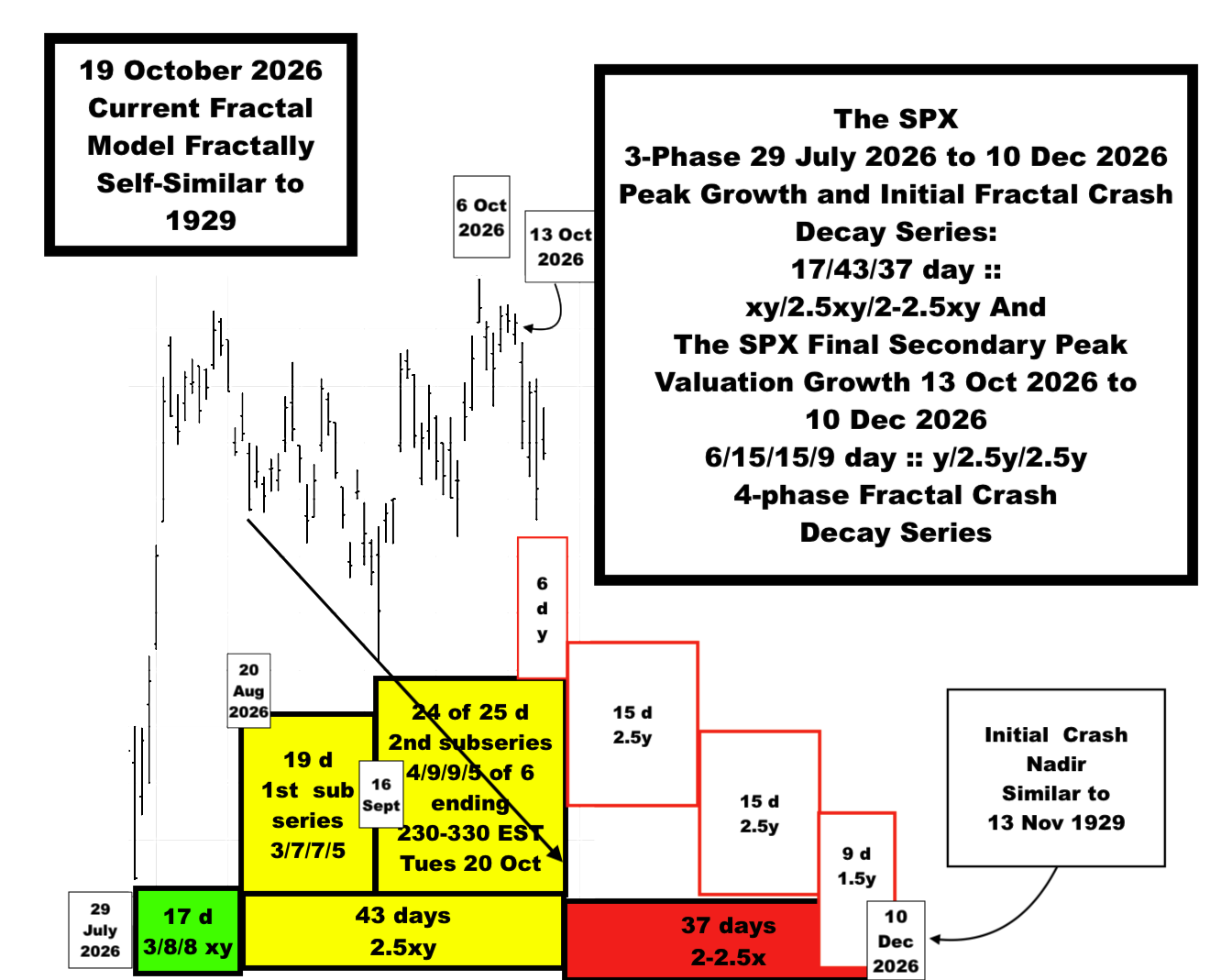
Above is the current Lammert 4-phase 30 March 2026 to 8 December 2026: 25/60/57/37 days :: x/2.5x/2-2.5x/1.5x that represents the terminal self-assembly growth of the SPX 1982 13/33-34 :: x/2.5x 1st and 2nd fractal series peaking 6 Oct 2026 and its initial crash decay nadir ending 8 December 2026. Interpolated within this 4-phase series are a 3-phase 30 March to 21 Oct 25/60/60 day :: x/2.5x/2.5x maximum fractal growth to final secondary peak valuation and a 9 October2026 6/15/15/9 day :: y/2.5y/2.5y/1.5y 4-phase Lammert Decay Fractal Series ending on 8 December 2026.
The US hegemonic asset-debt macroeconomic system is following a 1807 36/90/90/54-57 year :: x/2.5x/2.5x/1.5-1.6x Lammert4-phase fractal cycle. The 36 year 1st fractal ended in 1842-43; the 90 year 2nd fractal ended in 1932. The 90 year 3rd fractal and 54-57 year 4th fractal are self assembled and interpolated into a progressive logical fractal series from 1932 to 1982 with a terminal 1982 13/33-34/33-34/20 year :: x/2.5x/2.5x/1.5x fractal series ending 2074 to 2077. The interpolated 3rd fractal 90 year high occurred in Nov 2021. Unprecedented historically high peacetime annual US governmental deficit spending to GDP ratios and an explosive, enormous final private debt funded Chip/ LLM/AI/Data Center expansion propelled the SPX to higher valuations than the 3rd fractal 90 year high and finally to its 6 October 2026 all time high valuation at 7844.52. Estimated near-term revenues do not support AI- Et al. market valuations.
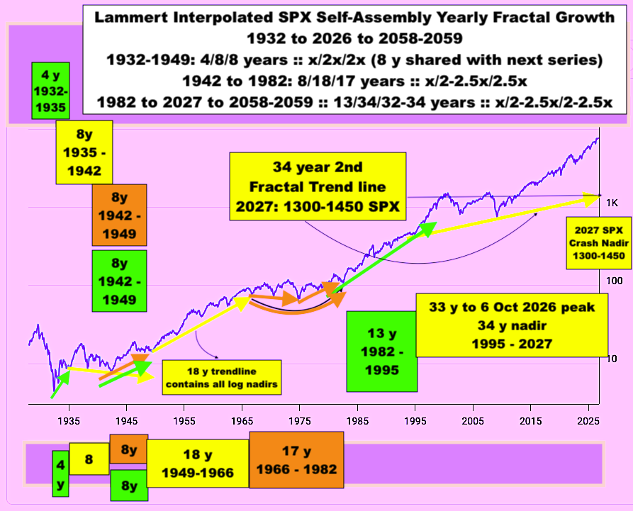
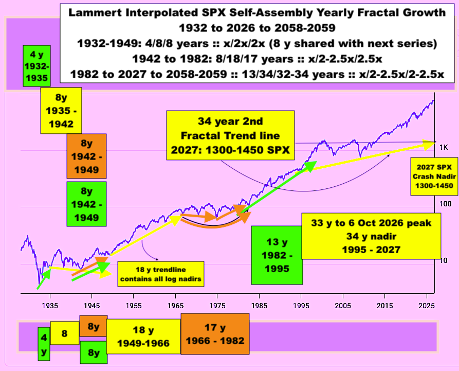
Below is a reposting of Lammert Fractal Progression since 1932. By underlying fractal trendlines, the SPX will nadir at 1300-1450 in 2027.
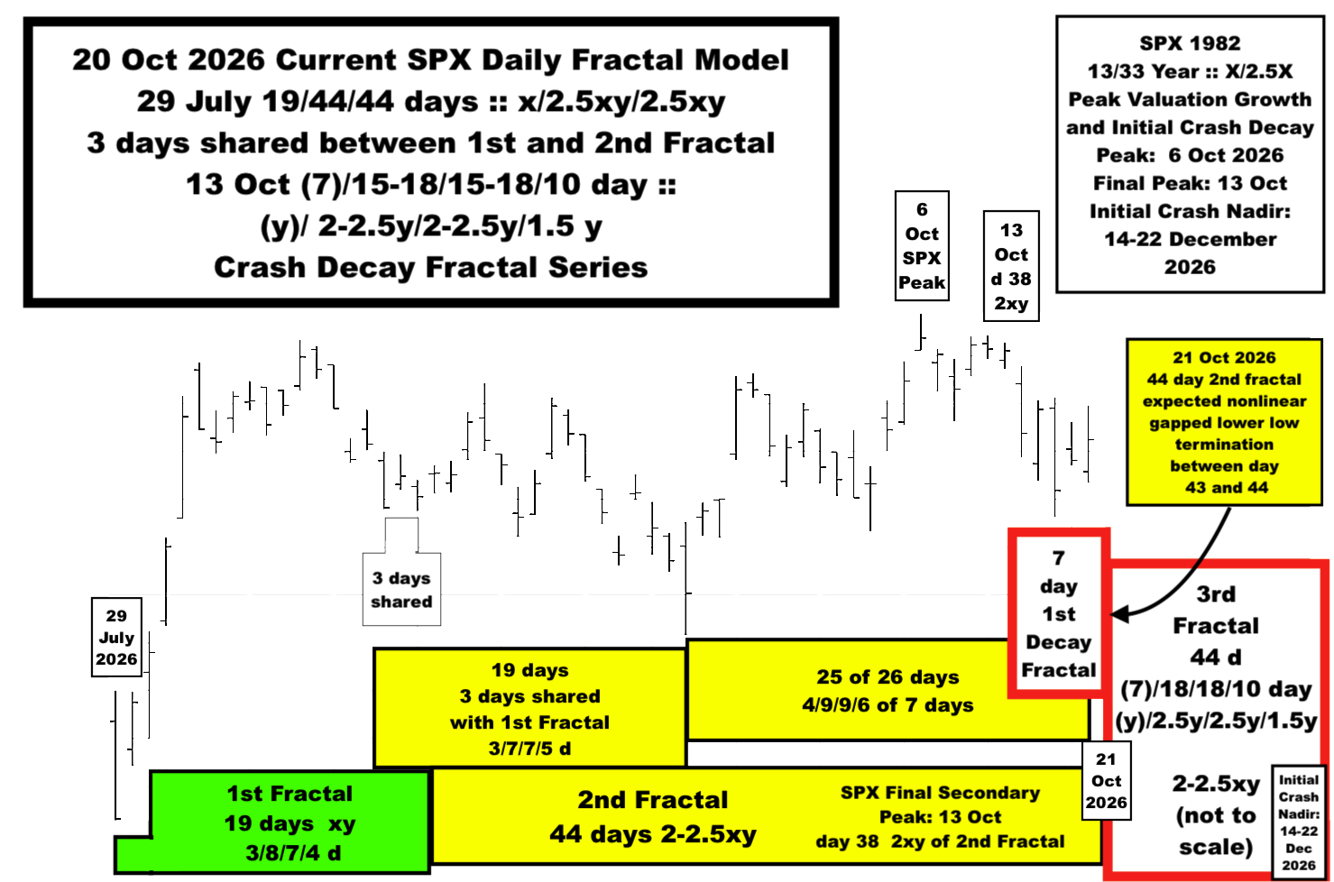
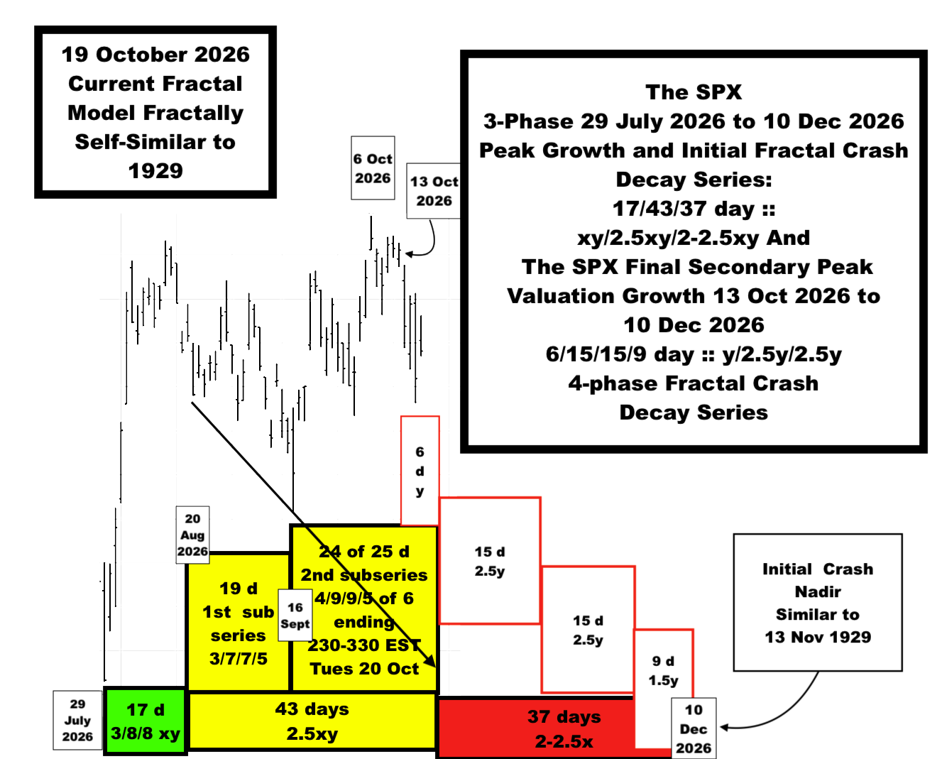
Above is the current Lammert fractal model of the SPX 29 July 2026 19/43 of 44/38-44 day :: xy/2-2.5xy/2-2.5xy 6 October 2026 all-time peak valuation and final peak high 13 Oct 7/15-18/15-10/10 day :: y/2-2.5y/2-2.5y/1.5y initial crash decay series ending 14-22 December 2026. In this fractal model, 3 days are shared between the 1st and 2nd fractals. 20 December is the 43rd day of the 2nd fractal. The final secondary peak on 13 Oct on day 38 of the 2nd fractal is a 2xy ratio of the 19 day :: xy 1st fractal.
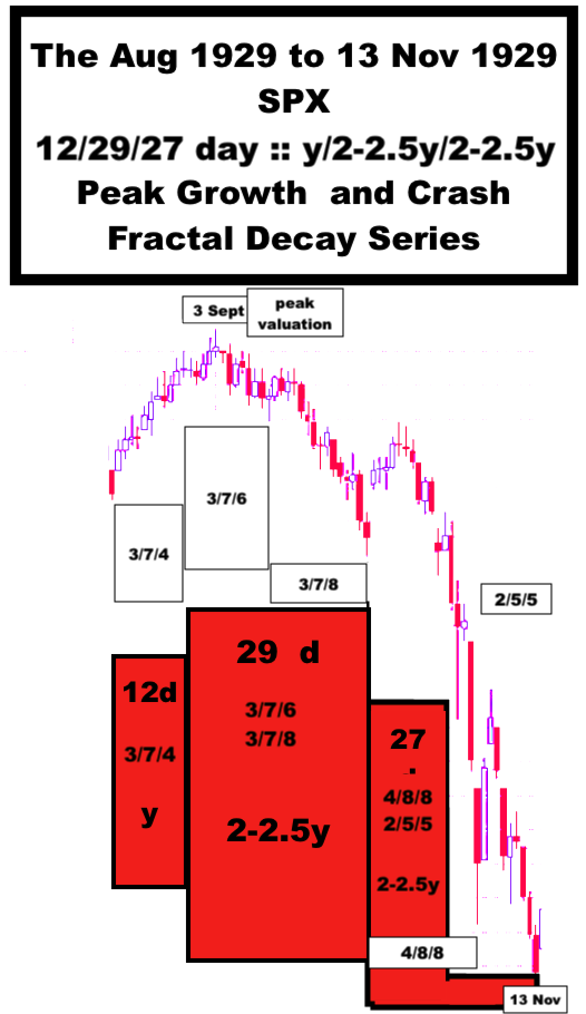
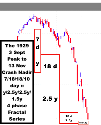
Below is the fractally self similar 1929 peak valuation and initial crash fractal decay series peaking on 3 September 1929 with an initial crash nadir on 13 November 1929.
The US hegemonic asset-debt macroeconomy is characterized by the recognizable periodic growth and decay of the valuation its progenitor and continuity stocks and commodities.
This website argues that their are two extremely regular time-unit-based fractal patterns governing a asset-debt system deterministic self-ordering, self-assembly process: a three phase fractal series: x/2-2.5x/1.5-2.5x and a four phase fractal series: x/2-2.5x/2-2.5x/1.5x-1.6x. Generally the individual fractal units are determined by their nadir points with the exception of the 3rd 2-2.5x fractal in the 4-phase series which can be a peak or terminal secondary peak valuation.
Within the easily recognizable fractal cycles, there are time limits to extreme credit expansion, extreme overvaluation, and extreme asset over production. When American companies made the primary goal of their businesses, profitability for their stockholders, considerations for the working middle class who support their enterprises and for investment for the well-being and continuity of the nation’s long term self interest were minimized. With the focus on profits for shareholders, buybacks, an no national strategic goals, valuation growth of equities now occurs to the maximum valuation fractal time extent; increasing wealth disparity is apparent.
The US hegemonic asset debt macroeconomic system is following an 1807 4-phase x/2.5x/2.5x/1.5-1.6x :: 36/90/90/54-57 year series ending in about 2077. Equity/commodity valuation 36 year 1st fractal and 90 year 2nd fractal nadirs occurred in 1841-42 and 1932, respectively, with a 90 year (2.5x) 3rd fractal peak in Nov 2021. Historically high average 7-9% peace-time deficit to GDP spending from 2020 to 2026 and recently AI/chip/data center large private investment has extended an interpolated 1932 SPX fractal series to the 6 Oct 2026 peak valuation.
The 1932 to 2077 90 year 2.5x 3rd fractal and the 54-57 year 1.5-1.6x 4th fractal are composed of two interpolated fractal series one complex fractal series from 1932 to 1982 and one from 1982 to 2077.
In past posts, the 1932 to 1982 fcomplex fracta series was described as a 10-11/20-22/20-22 year :: x/2x/2x fractal series ending in 1982.
The above graph shows a 1932 4/8/8 year ::x/2x/2x fractal series ending in 1949. The 1942 to 1949 8 year 3rd fractal is not in the 4/8 year x/2x 1st and 2nd fractal slope line. With America protected from destruction by two oceans and friendly neighbors, 20+% deficit to GDP spending and winning the war, the 1942 to 1949 8 year 3rd fractal is upsloping and becomes the 1st fractal of a 8/18/17 year :: x/2-2.5x/2-2.x fractal series with an 18 year 2-2.5x 2nd fractal nadir ending in 1966 and a 17 year 2-2.5x nadir ending in 1982. Note that the trend line from the beginning of 8 1st year fractal to the end of the 18 year 2nd fractal contain all intervening valuations.
In 1982 a 13/33 of 34 year :: x/2.5x (1982 to 2027) 1st and 2nd fractal series are self ordered. The SPX peak valuation of this series occurred during the 33 rd year 2.5x of the 33 year 2nd fractal on 6 October 2026. The 34 year 2027 SPX second fractal nadir valuation is expected to touch the March 2009 2nd fractal trendine for a low of 1300 to 1450, 81 to 84% lower than the peak valuation on 6 Oct 2026 at 7844.52.
The 19 Oct 2026 Current Peak Valuation to Initial Crash Decay Fractal Model:
29 July 2026 to 10 December 2026: 17/42 of 43/37 days :: xy/2.5xy/2-2.5 xy
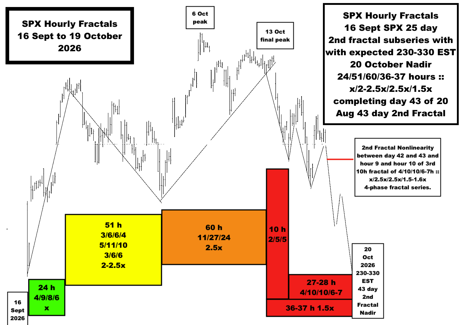
The 17 day 1st fractal is composed of a 3/8/8 day :: x/2.5x/2.5x 3-phase fractal series. Tomorrow is day 43 of the 43 day 2nd fractal. A nonlinear gapped lower low from Monday’s close will be evident at the opening as the extreme terminal 2x-2.5x portion of the 43 day 2nd fractal. The 43 day 2nd fractal is composed of two fractal series: a 20 Aug 2026 4-phase series: 19 day 3/7/7/5 day :: x2-2.5x/2.5x/1.6x and a 16 Sept 2026 4-phase 25 day 4/9/9/6 day :: x/2-2.5x/2-2.5x/1.5 x series ending with an expected nadir at 230 to 330 EST 20 October 2020. The all time SPX peak at 7844 .52 occurred on 6 October 2026 day 4 of the 9 day 3rd fractal. The secondary SPX peak valuation occurred on 12 Oct with a final secondary peak occurred on 13 Oct.
The 4 day 1st fractal of the 16 Sept 2026 4/9/9/6 day :: x/2-2.5x/2-2.5x/1.5x series is a 4-phase curvilinear blow-off fractal series of 25 hours 4/10/8/6 hrs :: x/2.5x/2x/1.5x ending at 930EST 22 September at a interday high valuation. The hourly fractal correlate series to the 4/9/9/6 daily fractal series is 24/51/60/36-37 hours :: x/2-2.5x/2.5x/1.5x. The last 36 hour 4th fractal is interpolated in two fractal series : an 1130 AM 13 October 3/6/6 hour :: x/2x/2x fractal series that contains the final 13 Oct 2026 tertiary high valuation and a final 930 EST 15 Oct 2026 4/10/10/6-7 hour :: x/2.5x/2.5x/1.5-1.6x 4-phase fractal series expected to nadir at 230-330 EST 20 October 2026 and completing the 43 day 2nd fractal.
The 16 September 24/51/60/36-37 hour :: x/2-2.5x/2.5x/1.5x terminal portion of the 43 day 2nd second fractal is self-similar to the 30 March 2026 to 10 December 2026 25/60/59/37 day :: x/2-2.5x/2-2.5x/1.5x 4-phase fractal series.
The 37 day 3rd fractal of the 29 July 2026 17/43/37 day tertiary peak growth and initial crash decay series is composed of a 13 Oct 2026 (6)/15/15/9 day (y)/2.5y/2.5y/1.5y series ending 10 December 2026 self similar to the 3 Sept 1929 7/18/18/10 day :: y/2.5y/2.5y/1.5y series ending 13 November 1929 peak growth and initial crash decay series.
19 October 2023Alternative Initial Crash Fractal Decay Model: a 12 Oct 7/15-18/15-18/9-10 day (y)/2-2.5y/2-2.5y/1.5y model ending in December 2026.